YouTube Channel: Mechanical Behavior of Materials

Please do visit my YouTube Channel which deals with a basic course on Mechanical Behavior of Materials.

Here, we will learn about the mechanical behavior of materials, linking their atomistic mechanism to their macroscopic behavior. We will deal with the continuum mechanics in view of the elastic and plastic behavior of materials. We will study the creep, fatigue, and fracture of materials. We will enquire together about “why do materials behave in a particular way as they do?

Please do comment/criticize and provide your suggestions to make it better. Your suggestions/advice/criticism are appreciated.

Zero-Creep experiment

The quantification of grain boundary energies and surface energies of materials is essential and its knowledge is important for many metallurgical processes such as sintering, solidification, grain boundary engineering, plastic-deformation and microstructure evaluation (texture etc.). Surface energies of the most of the solid materials can be evaluated using zero creep experiment which is one of the oldest and theoretically sound methods. The first zero creep experiment was done by Chapman and Porter in 1910 on gold foil [1]. Subsequently, this field was developed by major contributions of Udin et al., Maiya and Blakely, Miles and Leak and Josell et al.* [2-6]

In this post, a brief introduction to zero creep experiment and concept behind it is explained. This experiment is majorly carried out on the wires or foils for obtaining unambiguous results and to avoid complications during analysis.

The principle is based on the balancing of external applied (tensile) force to that of summation of energy associated with the grain of a sample. The schematic for such situation is shown in the following Figure.

At particular stress or zero creep stress (σ₀), the strain-rate becomes zero. At this situation, the system is in equilibrium.

Let us now understand the above scenario using bamboo shaped or cylindrical shaped grains having length “2L” and diameter “2R” as shown in the following Figure.

The surface energy per unit area and grain boundary energy per unit area of the cylindrical grain are designated as ‘γ_SF‘ and ‘γ_GB‘ respectively. Let the applied tensile load on the sample be ‘P’.

Then the free energy (F) of each grain is the total balance of surface energy, grain boundary energy and the potential energy due to an applied load.

Thus,

The ‘F’ mentioned here is analogous to the work of cohesion of the grain boundary interfaces. The work of cohesion in materials is decreased by grain boundaries and also by the potential energy due to applied load [7].

Thus, the above relation mathematically can be written as

 

At equilibrium i.e. at zero creep load (P₀) or zero creep stress (σ₀), F=0

 

Now, solving above equation for P₀, we get

Using Zero creep experiment, the stress at which there is no strain (or strain-rate=0) can be observed. From zero creep stress (σ₀) the zero creep load (P₀) can be obtained using the dimensions of the sample.

The ratio “2L/R” is obtained by direct measurements of the grain dimensions. However, the ratio “γ_GB/γ_FS” can be obtained by studying grain boundary grooves (refer the Following diagram).

Now, after knowing P₀, “2L/R” and “γ_GB/γ_FS”, one can evaluate surface energy ‘γ_FS’ from above relation. From ‘γ_FS’, the grain boundary energy ‘γ_GB’ can be obtained.

In this post, heuristic and simple ways are used to introduce ‘Zero-creep experiment’ which is its sole purpose. However, one can deal with more sophisticated and accurate analysis by referring the appropriate literature.

References:

1. JC Chapman, HL Porter, Proc. Roy. Soc. London A 83 (1910) 65.
2. H Udin. AJ Shaller, J Wulff, Trans AIME 185 (1949) 186.
3. H Udin, Trans AIME 191 (1951) 63.
4. PS Maiya, JM Blakely, JAP 38 (1967) 698.
5. B Mills, GM Leak, Acta Matell 16 (1968) 303.
6. D Josell, Acta Matell Mate. 41 (1993) 2179.
7. RJ Stokes, DF Evans, Fundamentals of Interfacial Engineering, John Wiley & Sons (1997).

*I haven’t mentioned all the researchers, for further reading please refer back references of the references mentioned above.

Acknowledgement: I thank Lavanya Raman for encouraging me to write on this topic.

γ (gamma)-Surface

γ-surface is one of the important concepts to understand the deformation behavior of the materials. It is also an important tool to visualize the dislocation core structures and in principle to understand stacking faults (SFs), antiphase-boundaries (APBs) and other surface defects. In this post, the concept of γ-surface has been introduced.

γ-surface, as the name suggests has to do something with the surface of the crystals/materials. Generally, for surface energy, the Greek letter γ is used {Vitek, V., Cryst. Lattice Defects 5 (1975) p. 1}.

So what is this γ-surface? How is it different from surface energy or grain-boundary energy? (Note: surface energy interchangeably used as surface tension and or interfacial energy, still ambiguity in the literature about the usage of these terms) Now why it is important to introduce and understand γ-surface? These are the obvious questions.

Let’s now brush-up some terminologies. A surface is the interface between solid and vacuum and can be quantified using surface energy. A grain boundary is the planar defect (2-D defect) created by the change in the orientations of the grains of the same material.

Now visualize the perfect crystal. Perfect means no defects at all. Consider a hypothetical plane as shown in the following figure. Now move* the upper part of the crystal above this plane relative to the lower part (*hereafter “translation” will be used for the movement). As we have assumed perfect crystal, we have an infinite array of atoms/molecules (motifs). Also, we know that the crystalline materials are bonded by ionic, covalent or metallic bonds. Thus there is an existence of a periodic potential between two halves of the crystal.  The translation on glide plane disturbs this potential and results in a change of energy which leads to the formation of “energy-surface”. We can translate the upper part relative to the lower part by a magnitude of vector lying in this glide plane. Thus, now this newly formed energy-surface needs an introduction; as it can’t be expressed using surface energy or grain boundary energy. With these understandings, we can define that the energy surface results from considering all possible translations lying in a given lattice plane is called γ-surface or generalized stacking fault energy (GSFEs).

                      

To understand γ-surface more clearly, let’s consider the simple cubic crystal structure. Consider (100) plane and glide plane as (002). Translate the upper part of glide plane along Y-direction.

With glide on (002) plane and translation along [010] direction, the variation in the energy is as shown in the following figure.

Now we know during deformation, the elastic energy is dependent directly on a square of the Burgers vector. Thus only those Burgers vectors are chosen that connect neighbouring absolute minima (or/ neighbouring saddle points) of the γ-surface.

In this post, an attempt was made to introduce γ-surface. It is but obvious and intriguing that the γ-surface will be different for different planes. It depends on the nature of bonding on that plane for a particular material.

To visualize the γ-surface, please check this link

http://www.mpie.de/3045424/Solid-melt-gamma-surfaces

Acknowledgement: I would like to acknowledge Dr Ajeet Srivastav for discussions involved during understanding his work {Srivastav et al., Scripta Mater 98 (2015) p. 20} which led me to comprehend and appreciate the γ-surface concept.

Hexagonal system and Miller-Bravais notations: i=-(h+k)

In hexagonal lattice (and crystals) directions and planes are designated by the 4-index notations (hkil) called as Miller-Bravais (M-B) notation.

In this post, the importance of M-B notations and derivation for i=-(h+k) is discussed.

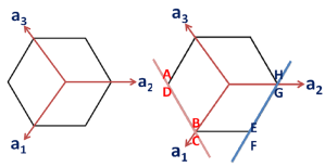
Before touching to the aforementioned problem, let’s understand the hexagonal system itself.

As we all know Miller indices of a hexagonal system are

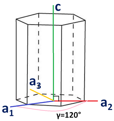
a=b≠c and α=β=90°, γ=120°

Please note that in the M-B notation (i.e. hkil)

• the first three indices (i.e. h, k and i) are symmetrically related (i.e. to a₁, a₂ and a₃ respectively) to the basal plane
• the third index (i) is a redundant one (i.e. can be derived from the first two and we will see the derivation of it in later part of this post)
• the fourth index (l) represents the ‘c’ axis (perpendicular to the basal plane)

The importance of the M-B notations is to clearly distinguish the family of planes and directions.

The M-B notations are introduced to make sure those members of a family of directions or planes are unambiguously identified.

Just check the following examples.

Consider the prismatic planes ABCD and EFGH. It is obvious and apparent from the following figure that these two planes belong to the same family (as they are parallel to common direction “c”).

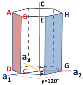
The following figures show the projections of these two planes on basal plane (with lattice parameters “a” and “c” i.e. |a₁|=|a₂|=|a₃|=a and |c|=c).

Check out the Miller indices for these two planes.

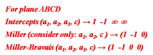
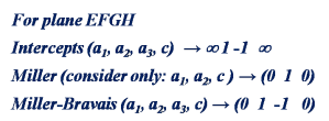
From the above example, it is clear that Miller indices indicate that these two planes are of a different family (even though they belong to the same family). But Miller-Bravais notations confirm that they are from the same family.

Now we will see the relation between the redundant index i with that of h and k, i.e. now we will derive relation i=-(h+k)

As the direction c is parallel to the direction z. So we will not worry, as index notation l in Bravais notations will be equal to that of Miller-Bravais index notation.

Now consider the basal plane and point X with indices hkil as shown in below figure. Here we will first derive a relation for a direction and same analogy can be extended to planes.

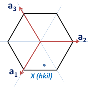
To find out the coordinates of point X i.e. the values of h, K and i in terms of a₁, a₂ and a₃. Thus we have to draw perpendiculars to these three axes which are shown in the below figure.

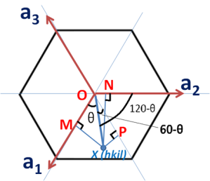
Let the distance OX=x units and then from the above figure

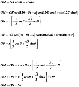
As from the above the direction of OP is opposite to that of a₃, thus as per the conventions

OM+ON=-OP

From figure we can say that, OM=h, ON=k and OP=-i

i.e. i=-(h+k)

This we have proved for the direction, with the same analogy, we can proceed for planes. In the case of planes, we have to consider intercept on the respective axis.

As mentioned earlier we are not bothered about the index in z direction as it is going to remain same in the M-B notations.

With this understanding, let us consider the plane (marked as a blue line in the following figure) cuts a₁ at A, a2 at B and a₃ at C.

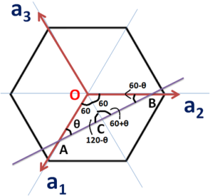
Thus by definition of Miller-indices (/M-B indices)

Now consider ∆OAC, and using law of sines, we can write following relations

Consider above expression as equation (1)

Similarly in ∆OCB,

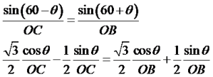
Consider above as equation (2)
Now, add equation (1) and (2)

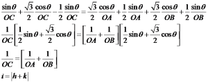
Now as direction of OC is opposite to that of a₃

Thus i=-(h+k)
Thus we have proved the relation for both directions and planes. Note that this relation is valid only for perfect hexagon system.

Maxwell relations

Maxwell relations find very important place to understand metallurgical thermodynamics and in turn most of the metallurgical processes. Maxwell relations are relations between second derivatives of the thermodynamic potentials.

Maxwell relations are listed below

Where P, T, S and V indicates pressure, temperature, entropy and volume respectively.

We will first see how to read these relations

 should be read as partial derivative of T with respect to V at constant Entropy S.

Similarly

should be read as partial derivative of P with respect to S at constant volume V.

The biggest problem is to remember these relations correctly.

In this post, we will see one method to remember these relations.

Look at the following square.

Difficult to remember this one. Try following square (it’s just for fun 🙂 )

Now look at the arrows marked carefully. They are diagonally marked. From P to V and S to T. Remember mark them in alphabetical order.

Now let’s write Maxwell equation.

Just concentrate on square.

Take partial derivative of P w.r.t. S

i.e.

As the derivative started with P. Thus this derivative will be always at constant volume V. Diagonally opposite term of the starting term. Here V is diagonally opposite of P (Another example, if T would have been the starting term then diagonal opposite is S). See the following square.

Now we are moving in the direction of the arrow i.e. from P to V, so the sign of the derivative of P w.r.t. S at constant V should be taken as positive (+Ve)

i.e. 

Now thermodynamically this term is equal to partial derivative of T w.r.t. V at constant S.

(See the green arrows for one to one correspondence of the terms)

Check the following square.

For , we are moving against of the arrow i.e. from T to S. Thus this term must be negative (-Ve).

i.e. 

Thus the first relation can be written as 

 

We just now have written first Maxwell relation mentioned at the start of the post.

Similarly, you can try to write other relations!

Semiconductors: Why ∆E≤3.2 eV ?

The materials are classified as metals, semiconductors and insulators based on the band gap theory. In metals, the valence and conduction band overlap and thus they are good conductors of heat and electricity. But in the case of semiconductors and insulators, there is a finite gap between the valence and conduction band. The band gap energy (∆E) is the energy difference between the valence and the conduction band of the material (in solid state). The following figure shows the classification of materials using energy band diagram. The unit of band gap energy is generally expressed in eV.

 

The materials are called semiconductors when ∆E≤3.2 eV (at T=0 K). If ∆E>3.2 eV, then the material is called as an insulator. Here we will see and try to understand, why the 3.2 eV is used as the criteria to say material as semiconductor or insulator.

As by definition of a semiconductor; when the sufficient energy is provided to these materials, the electrons from the valence band overcome the band gap energy and moves into the conduction band. Thus the electrical conductivity of semiconductor lies in between that of metals and insulators.

At 0 K condition, the energy available is from sunlight. The white light received on the Earth is comprised of radiations of variables wavelengths i.e. (visible spectrum) from violet (~400 nm) to red (~700 nm). Thus the maximum energy supplied by visible spectrum is through violet radiation.

The energy associated is given by

E=hν

Where E is energy (in J), h is Planck’s constant=6.63 × 10^-34 m² kg / s and ν is the frequency of the radiation where ν=c/λ, c=speed of light (3×10⁸ m/s) and λ is wavelength.

In the following calculation we have considered the λ= 400 nm (Violet)

To convert this energy from J into eV, we have to divide it by 1.6× 10^-19 (as 1 eV= 1.6× 10^-19 J)

Thus we get, E=3.11 eV

As the violet radiation is not monochromatic thus this energy supplied by violet radiation is assumed to be 3.2 eV (at T=0 K).

This is the energy available from sunlight and if it is sufficient to take of electrons of valence band to the conduction band of the materials, such materials are called semiconductors.

Dissociation of dislocation into partials in FCC crystal structure

In FCC crystal structure, the slip occurs on the {111} plane (as close-packed and highest atomic density) and in the <110> direction (highest atomic density in this direction).

However, it is very well understood that the Burger vector (a₀/2)[110] dissociates into partials creating stacking fault.

The dissociation reaction is as follows

                                                                                    (1)

Here we will try to derive this relationship with simple and basic understandings in geometry

Consider FCC crystal structure as shown below. The atoms are at corners of cube and face centres, the 111 plane is also shown.

 

 

 

 

 

 

 

Now focus only on the following lattice points

 

 

 

 

 

 

 

Check the tetrahedron OABC marked in the following diagram. It is called as Thomson’s Tetrahedron.

 

 

 

 

 

 

 

Consider the plane OBC as follows

 

 

 

 

 

 

 

We have to find out equation of the plane OBC. The equation of any plane can be written in the form

                                                                                               (2)

Now points O, B and C lie on this plane OBC. So they should satisfy the equation (2). Put coordinates of point O in the equation (2)

We get

d=0

Similarly put coordinates of B and C in equation (2), we get following values

a=-b and a=c

and now equation (2) becomes,

Using Millers Indices, the plane OBC is nothing but   plane

Now plane OBC is from the family of {111} which is slip plane for FCC

The direction BC is shortest lattice vector i.e. Burger’s vector for the FCC

Vector BC can be found as=coordinates of C – coordinates of B

The Vector BC using lattice vector a₀

                                                                                                                                (3)

Now as we know, BC dissociates into partials BD and DC (as shown in following figure). Point D lies on the plane OBC and is centroid of ∆OBC.

Consider the coordinates of D as D(x y z)

As D lies on plane OBC, it should satisfy the equation of the plane thus

x-y+z=0                                                                                                               (4)

Distance (BD) = Distance (DC)

Solving this we get, x=z                                                                                  (5)

Similarly
Distance (DO) = Distance (DC)

                                                                                                                                  (6)

by solving equations (4), (5) and (6)

Vector BD can be written as

                                                                                                                             (7)

Similarly

                                                                                                                            (8)

As per the law of vector addition, and from equation (7) & (8)

 

Derivation of Hooke’s Law

ut tensio, sic vis (The extension is proportional to force)

Prerequisite: Please brush-up terminologies Force, Stress, Tensile and compressive forces, stress, strain, elastic body, plastic body, Lennard-Jones potential

Hooke’s law states that the strain (ε) induced in the material is directly proportional to the stress applied (σ) in the elastic regime of the material.

E=σε

Where E is the proportionality constant and often referred as Young’s modulus when nature of force is tensile.

Derivation from the Material Engineers point of view

Consider two atoms separated at the distance ‘a’ apart from each other. When we try to bring them close to each other there are forces of attraction and forces of repulsion which play in. When the force of attraction is equal to the force of repulsion, system attains minimum energy. The distance is called equilibrium distance.

The total energy ‘U’ at any inter-atomic distance ‘a’ is given as the summation of attractive and repulsive energy

                                                                                                                                 (1)

 Where A, B, m and n are constants.

 quantifies attractive energy and second term  quantifies repulsive energy. Also note that m<n, then only atoms can attract each other.

Now try to recall this basis relationship

Energy=Force × displacement

Thus force F can be found out by differentiating equation (1)

                                                                                                      (2)

When a=a₀, Force of attraction and repulsion is equal.

i.e.

Find out the value of A

                                                                                                                             (3)

Put this value of A into the equation (2)

 

                                                                                            (4)

Using Lennard-Jones potential

                                                                                                             (5)

From equation (5), m=6 and n=12

And from equation (4)

In elastic regime of material

 and 

By definition of strain ε

Dividing both sides by area and assuming area to be a constant in elastic regime of the material,

we can get Stress, σ

and